Gravity in ORT#
In the first notebook, SRT was described by having everything move through spacetime at the speed of light \(c\). In this notebook we propose that near mass an escape velocity \(\vec{v}_{escape}\) arises. By adding the escape velocity to the spacetime motion, all gravitational effects follow:
When multiple masses are present, the escape velocities add as vectors. For a stationary object, therefore, \(c_{local} = \sqrt{c^2 - v_{escape}^2}\); for a moving object, \(c_{local}\) becomes direction-dependent through the dot product \(\vec{v}_{space} \cdot \vec{v}_{escape}\).
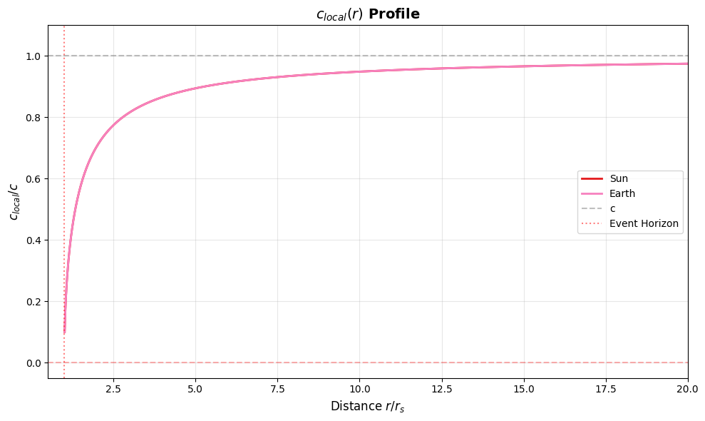
From this single extension — with \(c_{local}(r) = c \cdot \sqrt{1 - r_s/r}\) — all basic gravitational effects follow: time dilation, redshift, light deflection, orbital precession, and the full Schwarzschild metric.
import sys, pathlib
sys.path.insert(0, str(pathlib.Path().resolve().parent / 'shared'))
from ort_core import *
from ort_plots import (c_local_profile, c_local_profile_interactive, spacetime_embedding_3d,
    orbital_precession_plot, light_deflection_diagram, photon_sphere_shadow, einstein_ring_plot, comparison_table)
import matplotlib.pyplot as plt
import math
import numpy as np
%matplotlib inline
1 The principle: a position-dependent \(c_{local}\)#
Core principle: near mass an escape velocity \(\vec{v}_{escape}\) arises, directed away from the mass. By adding it to the spacetime motion, all gravitational effects follow — isotropic at rest, anisotropic in motion.
1.1 Escape velocity as a component#
In SRT everything moves at \(c\) through spacetime: \(v_{space}^2 + v_{time}^2 = c^2\). Near mass the escape velocity \(v_{escape} = \sqrt{2GM/r}\) adds to the spatial velocity:
Expanded with the dot product:
Two layers#
Isotropic (stationary, \(v_{space} = 0\)): the dot product vanishes and the three components are orthogonal (Pythagoras):
Both time dilation and spatial stretching are isotropic — independent of direction.
Anisotropic (moving, \(v_{space} \neq 0\)): the cross term \(2\,\vec{v}_{space} \cdot \vec{v}_{escape}\) makes the effect direction-dependent. Tangentially (\(\alpha = 90°\)) the dot product is zero; radially it is maximal.
The local spacetime velocity#
For a stationary object (\(v_{space} = 0\)) this is the local spacetime velocity:
For a moving object the available spacetime velocity also depends on direction — this is worked out in chapter 3.
# c_local profile for the Sun and the Earth
fig = c_local_profile([SUN, EARTH], ['Sun', 'Earth'], lang='en')
plt.show()
# Interactive: adjust the mass and view the c_local profile
c_local_profile_interactive(lang='en')
Interactive version — download the notebook to use the slider.
1.2 The gradient of \(c_{local}\)#
The derivative of formula (1) with respect to \(r\):
Multiplied by \(c\):
For \(r \gg r_s\) this yields Newton’s \(g = GM/r^2\). The slope of the \(c_{local}\) field is proportional to gravity. This derivation applies to a stationary object (\(v_{space} = 0\)) — the isotropic case from §1.1.
# Verification: c · dc_local/dr = g
print("=== Gradient of c_local = gravity ===")
print()

# Earth
print("--- Earth (surface) ---")
dc_dr_earth = EARTH.dc_local_dr(R_EARTH)
g_earth = EARTH.proper_acceleration(R_EARTH)
print(f"  dc_local/dr      = {dc_dr_earth:.6e} [1/s]")
print(f"  g                = {g_earth:.4f} m/s²")
print(f"  c · dc_local/dr  = {dc_dr_earth * C:.4f} m/s²")
print(f"  Ratio            = {dc_dr_earth * C / g_earth:.15f}  (should be 1)")
print()

# Sun
print("--- Sun (surface) ---")
dc_dr_sun = SUN.dc_local_dr(R_SUN)
g_sun = SUN.proper_acceleration(R_SUN)
print(f"  dc_local/dr      = {dc_dr_sun:.6e} [1/s]")
print(f"  g                = {g_sun:.4f} m/s²")
print(f"  c · dc_local/dr  = {dc_dr_sun * C:.4f} m/s²")
print(f"  Ratio            = {dc_dr_sun * C / g_sun:.15f}")
print()

# Black hole (10 M☉) — strong field
BH = GravityModel(10 * M_SUN)
print("--- Black hole 10 M☉ (r = 1.1 r_s) ---")
r_bh = 1.1 * BH.rs
dc_dr_bh = BH.dc_local_dr(r_bh)
g_bh = BH.proper_acceleration(r_bh)
print(f"  dc_local/dr      = {dc_dr_bh:.6e} [1/s]")
print(f"  g                = {g_bh:.6e} m/s²")
print(f"  c · dc_local/dr  = {dc_dr_bh * C:.6e} m/s²")
print(f"  Ratio            = {dc_dr_bh * C / g_bh:.15f}")
print()
print("The relation c · dc_local/dr = g holds EXACTLY, from weak to strong field.")
=== Gradient of c_local = gravity ===

--- Earth (surface) ---
  dc_local/dr      = 3.275591e-08 [1/s]
  g                = 9.8200 m/s²
  c · dc_local/dr  = 9.8200 m/s²
  Ratio            = 1.000000000000000  (should be 1)

--- Sun (surface) ---
  dc_local/dr      = 9.149065e-07 [1/s]
  g                = 274.2821 m/s²
  c · dc_local/dr  = 274.2821 m/s²
  Ratio            = 1.000000000000000

--- Black hole 10 M☉ (r = 1.1 r_s) ---
  dc_local/dr      = 1.390825e+04 [1/s]
  g                = 4.169589e+12 m/s²
  c · dc_local/dr  = 4.169589e+12 m/s²
  Ratio            = 1.000000000000000

The relation c · dc_local/dr = g holds EXACTLY, from weak to strong field.
Derivation via GRT#
GRT derives \(g\) as follows:
Step |
GRT |
ORT (\(v_{space} = 0\)) |
Meaning |
|---|---|---|---|
1. Metric |
\(f(r) = 1 - r_s/r\) |
\((c_{local}/c)^2\) |
Shape of spacetime |
2. Four-velocity |
\(u^t = 1/\sqrt{f}\) |
\(c/c_{local}\) |
How fast time ticks |
3. Christoffel symbol |
\(\Gamma^r_{tt} = f \cdot GM/r^2\) |
\(dc_{local}/dr\) |
How fast the field changes |
4. Geodesic equation |
\(a^r_{coord} = -GM/r^2\) |
idem: \(-GM/r^2\) |
Coordinate acceleration |
5. Frame projection |
\(\times 1/\sqrt{f}\) |
\(\times c/c_{local}\) |
From coordinates to local |
Same result. GRT via differential geometry, ORT via the gradient of \(c_{local}\).
2 Time effects#
Core principle: as in the SRT part of ORT, everything moves at \(c\) through spacetime — but near mass \(\vec{v}_{escape}\) is added, so that for a stationary object \(c_{local}\) remains.
2.1 Gravitational time dilation#
At distance \(r\) from a mass, a clock has the local spacetime velocity \(c_{local} < c\). When the clock is stationary in space (\(v_{space} = 0\)), all of \(c_{local}\) goes to the time direction:
This is the Schwarzschild time dilation. The closer to the mass, the slower time runs.
# Time dilation at Earth's surface, GPS orbit, ISS orbit
print("=== Gravitational Time Dilation (Earth) ===")
print(f"Schwarzschild radius Earth: r_s = {EARTH.rs:.4e} m = {EARTH.rs*1000:.4f} mm")
print()

locations = [
    ("Earth surface", R_EARTH),
    ("ISS (408 km)", R_ISS),
    ("GPS (20,200 km)", R_GPS),
]
for name, r in locations:
    td = EARTH.time_dilation_factor(r)
    diff_per_day = (1 - td) * 86400e6  # microseconds per day
    print(f"{name:25s}: τ/t∞ = {td:.15f}  (offset: {diff_per_day:.3f} µs/day)")
=== Gravitational Time Dilation (Earth) ===
Schwarzschild radius Earth: r_s = 8.8698e-03 m = 8.8698 mm

Earth surface            : τ/t∞ = 0.999999999303892  (offset: 60.144 µs/day)
ISS (408 km)             : τ/t∞ = 0.999999999345788  (offset: 56.524 µs/day)
GPS (20,200 km)          : τ/t∞ = 0.999999999833092  (offset: 14.421 µs/day)
# Newton vs ORT: time dilation at GPS altitude
# Newton has NO time dilation — time is absolute!
r_gps = R_EARTH + 20_200_000  # GPS altitude ~20,200 km
td_ort = EARTH.time_dilation_factor(r_gps)
drift_per_day_us = (1 - td_ort) * 86400 * 1e6  # µs per day

print("=== Newton vs ORT: gravitational time dilation ===")
print(f"Clock at GPS altitude ({20200} km):")
print(f"  Newton:  Δt = 0 µs/day      (time is absolute!)")
print(f"  ORT:     Δt = {drift_per_day_us:+.2f} µs/day  (clock runs FASTER)")
print()
print(f"Without correction: GPS would drift {abs(drift_per_day_us) * C * 1e-6:.0f} m after 1 day!")
print(f"After 1 week: {abs(drift_per_day_us) * 7 * C * 1e-6:.0f} m — navigation useless.")
=== Newton vs ORT: gravitational time dilation ===
Clock at GPS altitude (20200 km):
  Newton:  Δt = 0 µs/day      (time is absolute!)
  ORT:     Δt = +14.42 µs/day  (clock runs FASTER)

Without correction: GPS would drift 4323 m after 1 day!
After 1 week: 30263 m — navigation useless.
2.2 Gravitational redshift#
Light emitted where \(c_{local}\) is lower has a lower frequency — where time ticks slower, the frequency is lower. A distant observer therefore measures a redshift:
# Pound-Rebka experiment (1959): 22.5 m height difference
h = 22.5  # meters
r_bottom = R_EARTH
r_top = R_EARTH + h

z = EARTH.gravitational_redshift(r_bottom, r_top)
delta_f_over_f = -z  # redshift = negative

# Approximation: Δf/f ≈ g·h/c²
g = G * M_EARTH / R_EARTH**2
approx = g * h / C**2

print("=== Pound-Rebka Experiment ===")
print(f"Height: {h} m")
print(f"Redshift z             = {z:.6e}")
print(f"|Δf/f|                 = {abs(delta_f_over_f):.6e}")
print(f"Approximation g·h/c²  = {approx:.6e}")
print(f"Measured (1959)        = (2.57 ± 0.26) ·10⁻¹⁵")
=== Pound-Rebka Experiment ===
Height: 22.5 m
Redshift z             = 2.442491e-15
|Δf/f|                 = 2.442491e-15
Approximation g·h/c²  = 2.458394e-15
Measured (1959)        = (2.57 ± 0.26) ·10⁻¹⁵
2.3 GPS: SRT + gravity combined#
A GPS satellite combines two effects: its velocity relative to the Earth’s surface and its position higher in the gravitational field both affect the clock rate.
Component |
Cause |
Effect |
|---|---|---|
SRT |
Satellite velocity (3870 m/s) |
−7 µs/day (slower) |
Gravity |
Higher \(c_{local}\) at GPS altitude |
+45 µs/day (faster) |
Net |
Combined |
+38 µs/day (faster) |
# GPS correction: combined SRT + gravity
v_gps = 3870  # m/s (GPS satellite velocity)

# Earth surface (at rest)
td_surface = EARTH.combined_time_dilation(R_EARTH, 0)

# GPS satellite (moving at altitude)
td_gps = EARTH.combined_time_dilation(R_GPS, v_gps)

# Difference in microseconds per day
diff_us_per_day = (td_gps - td_surface) * 86400 * 1e6

# Individual components
grav_only = (EARTH.time_dilation_factor(R_GPS) - EARTH.time_dilation_factor(R_EARTH)) * 86400 * 1e6
srt_only = (math.sqrt(1 - (v_gps/C)**2) - 1) * 86400 * 1e6

print("=== GPS Correction ===")
print(f"Gravity only:           {grav_only:+.2f} µs/day")
print(f"SRT only (velocity):    {srt_only:+.2f} µs/day")
print(f"Combined (formula):     {diff_us_per_day:+.2f} µs/day")
print(f"\nExpected net:           +38 µs/day")
=== GPS Correction ===
Gravity only:           +45.72 µs/day
SRT only (velocity):    -7.20 µs/day
Combined (formula):     +38.52 µs/day

Expected net:           +38 µs/day
2.4 The event horizon (\(c_{local} = 0\))#
At \(r = r_s\), \(v_{grav} = c\) and \(c_{local} = 0\). The consequences:
Nothing can move — neither through space nor through time
Clocks stop — \(v_{time} = 0\) for a stationary object
Light cannot escape — outgoing light has \(v = c - v_{grav} = 0\)
A freely falling object notices nothing special: \(\vec{v}_{space} = \vec{v}_{grav}\), so \(v_{time} = c\). It crosses the horizon in finite proper time — but the light it sends outward stands still.
# Black hole of 10 solar masses
BH_10 = GravityModel(10 * M_SUN)
print(f"=== Black hole of 10 M☉ ===")
print(f"r_s = {BH_10.rs:.3e} m = {BH_10.rs/1000:.2f} km")
print()

# c_local at various distances from the horizon
factors = [10.0, 5.0, 2.0, 1.5, 1.1, 1.01, 1.001, 1.0]
print(f"{'r/r_s':>8s}  {'c_local/c':>12s}  {'c_local (m/s)':>15s}")
print("-" * 40)
for f in factors:
    r = f * BH_10.rs
    cl = BH_10.c_local(r)
    print(f"{f:8.3f}  {cl/C:12.6f}  {cl:15.0f}")
=== Black hole of 10 M☉ ===
r_s = 2.954e+04 m = 29.54 km

   r/r_s     c_local/c    c_local (m/s)
----------------------------------------
  10.000      0.948683        284408098
   5.000      0.894427        268142526
   2.000      0.707107        211985280
   1.500      0.577350        173085256
   1.100      0.301511         90390827
   1.010      0.099504         29830465
   1.001      0.031607          9475533
   1.000      0.000000                0
3 Spatial effects#
Core principle: the escape velocity \(\vec{v}_{grav}\) is a vector — directed toward the mass. For a stationary object the effect is isotropic (time dilation), but for a moving object it depends on the angle: the dot product \(\vec{v}_{space} \cdot \vec{v}_{grav}\) determines the spatial anisotropy.
# v_grav at various distances
print("=== Velocity budget near 10 M☉ black hole ===")
print(f"{'r/r_s':>8s}  {'v_grav/c':>10s}  {'c_local/c':>10s}  {'check v²+c²':>12s}")
print("-" * 46)
for f in [10.0, 5.0, 2.0, 1.5, 1.1, 1.01, 1.0]:
    r = f * BH_10.rs
    vg = BH_10.v_grav(r)
    cl = BH_10.c_local(r)
    check = math.sqrt(vg**2 + cl**2) / C
    print(f"{f:8.3f}  {vg/C:10.6f}  {cl/C:10.6f}  {check:12.9f}")
=== Velocity budget near 10 M☉ black hole ===
   r/r_s    v_grav/c   c_local/c   check v²+c²
----------------------------------------------
  10.000    0.316228    0.948683   1.000000000
   5.000    0.447214    0.894427   1.000000000
   2.000    0.707107    0.707107   1.000000000
   1.500    0.816497    0.577350   1.000000000
   1.100    0.953463    0.301511   1.000000000
   1.010    0.995037    0.099504   1.000000000
   1.000    1.000000    0.000000   1.000000000
3.1 Spatial stretching#
Direction-dependent effects#
The full velocity budget is:
The dot product \(\vec{v}_{space} \cdot \vec{v}_{grav} = |v_{space}| \cdot |v_{grav}| \cdot \cos\alpha\), where \(\alpha\) is the angle between the direction of motion and \(\vec{v}_{grav}\).
Tangential (\(\alpha = 90°\), perpendicular to \(\vec{v}_{grav}\)): \(\cos\alpha = 0\), dot product vanishes.
Radially outward (\(\alpha = 180°\)): \((v_{space} + v_{grav})^2 + v_{time}^2 = c^2\)
Radially inward (\(\alpha = 0°\)): \((v_{space} - v_{grav})^2 + v_{time}^2 = c^2\)
This is the river model: space flows inward at \(v_{grav}\). Outgoing light swims against the current, incoming light is carried along.
Consequences for spatial stretching#
Spatial stretching is anisotropic — only in the radial direction:
Tangentially there is no stretching: the circumference at coordinate \(r\) is simply \(2\pi r\).
This follows directly from the vector nature of \(\vec{v}_{grav}\):
Radial: \(\vec{v}_{space}\) and \(\vec{v}_{grav}\) are parallel → linear interaction → extra effect
Tangential: \(\vec{v}_{space}\) and \(\vec{v}_{grav}\) are perpendicular → quadratic addition → only \(c_{local}\)
Both diagonal components#
Together with the time component from chapter 2:
Component |
Schwarzschild |
ORT |
|---|---|---|
Time (\(g_{tt}\)) |
\(1 - r_s/r\) |
\((c_{local}/c)^2\) |
Space (\(g_{rr}\)) |
\((1 - r_s/r)^{-1}\) |
\((c/c_{local})^2\) |
Angle (\(g_{\phi\phi}\)) |
\(r^2\) |
\(r^2\) |
ORT reproduces the full Schwarzschild metric. \(g_{tt} \cdot g_{rr} = 1\) — the two components are each other’s inverse. One principle (\(\vec{v}_{grav}\) as a vector) determines all three.
# Spatial stretching near the Sun and a 10 M☉ black hole
print("=== Spatial Stretching ===")
print()
print("--- Sun (surface) ---")
stretch_sun = SUN.spatial_stretching(R_SUN)
print(f"Stretching factor: {stretch_sun:.10f}")
print(f"Extra length per km: {(stretch_sun - 1) * 1000:.6f} m")
print()
print("--- 10 M☉ black hole ---")
for f in [10.0, 3.0, 1.5, 1.1, 1.01]:
    r = f * BH_10.rs
    s = BH_10.spatial_stretching(r)
    print(f"  r = {f:.2f} r_s:  stretching = {s:.6f}  (1 km → {s:.6f} km)")
=== Spatial Stretching ===

--- Sun (surface) ---
Stretching factor: 1.0000021231
Extra length per km: 0.002123 m

--- 10 M☉ black hole ---
  r = 10.00 r_s:  stretching = 1.054093  (1 km → 1.054093 km)
  r = 3.00 r_s:  stretching = 1.224745  (1 km → 1.224745 km)
  r = 1.50 r_s:  stretching = 1.732051  (1 km → 1.732051 km)
  r = 1.10 r_s:  stretching = 3.316625  (1 km → 3.316625 km)
  r = 1.01 r_s:  stretching = 10.049876  (1 km → 10.049876 km)
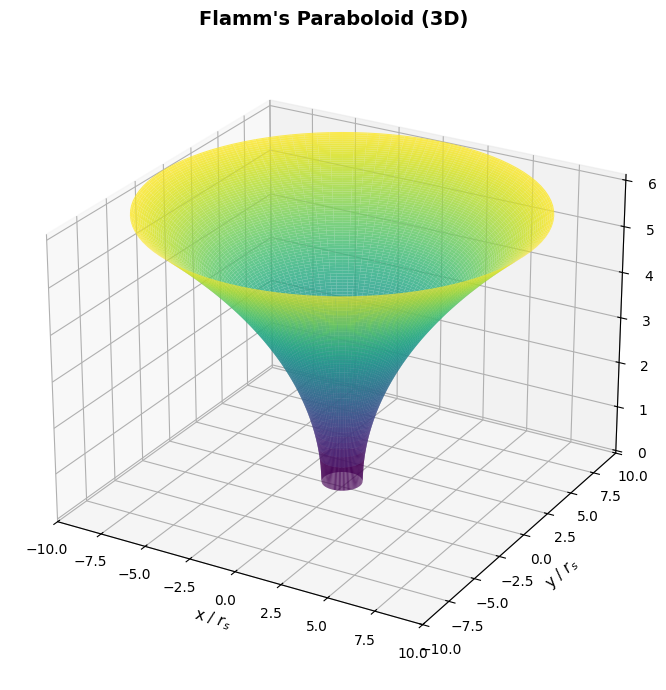
Flamm’s paraboloid#
Spatial stretching is traditionally visualized as Flamm’s paraboloid: a 2D embedding of the equatorial plane in 3D. The extra dimension (z-axis) is a mathematical device — not a physical direction — showing how much radial distance is stretched.
Because ORT gives the same radial stretching (\(g_{rr} = (c/c_{local})^2\)) and the same tangential geometry (\(g_{\phi\phi} = r^2\), circumference = \(2\pi r\)) as the Schwarzschild metric, Flamm’s paraboloid is also the correct visualization of ORT.
# 3D embedding of the spatial geometry
fig = spacetime_embedding_3d(lang='en')
if fig is not None:
    fig.show()
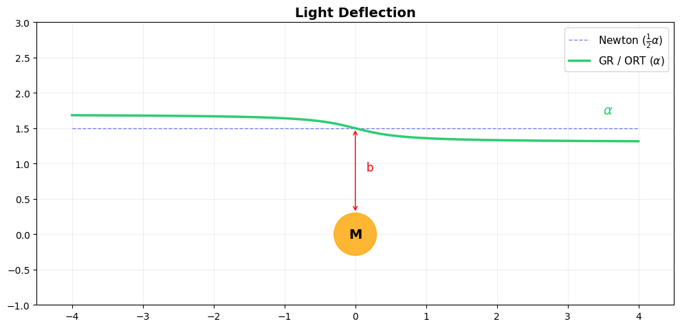
3.2 Light deflection#
Light grazing a mass is deflected. The deflection comes from two effects:
Time dilation (\(c_{local} < c\)): light moves locally slower → deflects as in a refractive medium
Radial stretching (dot product \(\vec{v}_{space} \cdot \vec{v}_{grav}\)): the radial component of the light path experiences extra delay
Both contributions are equal. The effective refractive index for a radial light path:
The total deflection angle:
This is the GRT result (Einstein 1915: 1.75”). Soldner (1801) and Einstein (1911) found half: only the time effect, without the radial stretching.
# Light deflection diagram
fig = light_deflection_diagram(lang='en')
plt.show()
# Light deflection by the Sun (b = R_sun)
alpha_arcsec = SUN.light_deflection_arcsec(R_SUN)
alpha_half = SUN.half_light_deflection(R_SUN) * (180/math.pi) * 3600

print("=== Light Deflection by the Sun ===")
print(f"Impact parameter b = R_sun = {R_SUN:.3e} m")
print(f"Soldner/Einstein 1911 (half value): {alpha_half:.4f}\"")
print(f"ORT / GRT (full):       {alpha_arcsec:.4f}\"")
print(f"Measured (Eddington 1919):          1.75 ± 0.06\"")
=== Light Deflection by the Sun ===
Impact parameter b = R_sun = 6.957e+08 m
Soldner/Einstein 1911 (half value): 0.8759"
ORT / GRT (full):       1.7517"
Measured (Eddington 1919):          1.75 ± 0.06"
# Newton vs ORT: light deflection by the Sun
# Newton/Soldner (1801) predicts HALF the correct answer!
alpha_newton = SUN.half_light_deflection(R_SUN) * (180 / math.pi) * 3600
alpha_ort = SUN.light_deflection_arcsec(R_SUN)

print("=== Newton vs ORT: light deflection by the Sun ===")
print(f"  Newton/Soldner (1801):  {alpha_newton:.4f}\"  (time curvature only)")
print(f"  ORT/Einstein (1915):    {alpha_ort:.4f}\"  (time + space curvature)")
print(f"  Eddington (1919):       1.75 ± 0.06\"  (measured!)")
print()
print(f"Newton predicts exactly HALF: {alpha_newton/alpha_ort:.3f}×")
print(f"The missing half comes from spatial curvature — something Newton lacks.")
=== Newton vs ORT: light deflection by the Sun ===
  Newton/Soldner (1801):  0.8759"  (time curvature only)
  ORT/Einstein (1915):    1.7517"  (time + space curvature)
  Eddington (1919):       1.75 ± 0.06"  (measured!)

Newton predicts exactly HALF: 0.500×
The missing half comes from spatial curvature — something Newton lacks.
3.3 Orbital precession#
In Newton the effective potential yields a closed ellipse — no precession. In ORT an extra term appears due to radial stretching:
Just as with light deflection, the precession comes from two contributions:
Time dilation (\(g_{tt}\)): varying clock rate
Radial stretching (\(g_{rr}\)): the dot product \(\vec{v}_{space} \cdot \vec{v}_{grav}\) affects the radial component of the orbit
Combined:
Mercury — the classical test#
For Mercury: \(\Delta\varphi\) = 42.98”/century — exactly the observed value (Le Verrier 1859, Einstein 1915).
Planet |
Δφ/orbit (“) |
Orbits/century |
Δφ/century (“) |
Observed (“) |
|---|---|---|---|---|
Mercury |
0.1035 |
415.2 |
42.98 |
43.0 |
Venus |
0.0053 |
162.5 |
0.86 |
8.6* |
Earth |
0.0038 |
100.0 |
0.38 |
3.8* |
* Observed values also include gravitational influences from other planets.
# Orbital precession of Mercury
prec_per_orbit = SUN.orbital_precession_arcsec(A_MERCURY, E_MERCURY)
prec_per_century = SUN.orbital_precession_arcsec_century(A_MERCURY, E_MERCURY, T_MERCURY)

print("=== Orbital Precession of Mercury ===")
print(f"Semi-major axis a = {A_MERCURY:.4e} m")
print(f"Eccentricity e    = {E_MERCURY}")
print(f"Orbital period    = {T_MERCURY/86400:.3f} days")
print(f"\nΔφ per orbit       = {prec_per_orbit:.4f}\"")
print(f"Δφ per century     = {prec_per_century:.2f}\"")
print(f"Observed          = 43.0\"")
=== Orbital Precession of Mercury ===
Semi-major axis a = 5.7909e+10 m
Eccentricity e    = 0.20563
Orbital period    = 87.969 days

Δφ per orbit       = 0.1035"
Δφ per century     = 42.99"
Observed          = 43.0"
# Newton vs ORT: orbital precession of Mercury
# Newton predicts closed ellipses — 0 extra precession!
prec_ort = SUN.orbital_precession_arcsec(A_MERCURY, E_MERCURY)
prec_per_century = prec_ort * (100 * 365.25 * 86400) / T_MERCURY

print("=== Newton vs ORT: orbital precession of Mercury ===")
print(f"  Newton:           0.00\"/century  (ellipse closes exactly!)")
print(f"  ORT/Einstein:    {prec_per_century:.2f}\"/century")
print(f"  Observed:        43.0 ± 0.1\"/century  (Le Verrier, 1859)")
print()
print(f"This unexplained discrepancy was a mystery for 56 years.")
print(f"Einstein solved it in 1915 — his first confirmation of GRT.")
=== Newton vs ORT: orbital precession of Mercury ===
  Newton:           0.00"/century  (ellipse closes exactly!)
  ORT/Einstein:    42.99"/century
  Observed:        43.0 ± 0.1"/century  (Le Verrier, 1859)

This unexplained discrepancy was a mystery for 56 years.
Einstein solved it in 1915 — his first confirmation of GRT.
# Precession plot for Mercury
fig = orbital_precession_plot(SUN, A_MERCURY, E_MERCURY, n_orbits=5, lang='en')
plt.show()

4 The complete picture#
Core principle: everything moves at \(c\) through spacetime. Near mass, part goes to the escape velocity \(\vec{v}_{grav}\), directed toward the mass. For a stationary object the effect is isotropic (time dilation), for a moving object it depends on direction (spatial anisotropy via the dot product).
Five effects from one principle:
Clocks run slower where \(c_{local}\) is lower → time dilation (isotropic)
Space stretches radially through the dot product \(\vec{v}_{space} \cdot \vec{v}_{grav}\) → anisotropic stretching
Light deflects due to time dilation + radial stretching (each half)
Light shifts to lower frequency → redshift
At \(v_{grav} = c\) everything stops → event horizon
4.1 The Schwarzschild connection#
The Schwarzschild metric for a spherically symmetric mass:
ORT reproduces all three components:
Schwarzschild |
ORT |
Origin |
|
|---|---|---|---|
Time: \(g_{tt}\) |
\(1 - r_s/r\) |
\((c_{local}/c)^2\) |
\(v_{space} = 0\): dot product vanishes |
Space: \(g_{rr}\) |
\((1 - r_s/r)^{-1}\) |
\((c/c_{local})^2\) |
\(\vec{v}_{space} \parallel \vec{v}_{grav}\): linear interaction |
Angle: \(g_{\phi\phi}\) |
\(r^2\) |
\(r^2\) |
\(\vec{v}_{space} \perp \vec{v}_{grav}\): dot product zero |
The agreement is not approximate — it is an exact equality. The vector nature of \(\vec{v}_{grav}\) determines all three metric components.
# Numerical verification: g_tt and g_rr from Schwarzschild vs from c_local/c
print("=== Schwarzschild verification: g_tt and g_rr from c_local ===")
print()
print(f"{'r/r_s':>8s}  {'g_tt (Schw)':>12s}  {'(c_l/c)²':>12s}  {'g_rr (Schw)':>12s}  {'(c/c_l)²':>12s}  {'match':>6s}")
print("-" * 70)
for f in [100.0, 10.0, 5.0, 3.0, 2.0, 1.5, 1.1, 1.01]:
    r = f * BH_10.rs
    # Schwarzschild metric components
    g_tt_schw = 1 - BH_10.rs / r
    g_rr_schw = 1 / (1 - BH_10.rs / r)
    # ORT: from c_local
    cl = BH_10.c_local(r)
    g_tt_ort = (cl / C) ** 2
    g_rr_ort = (C / cl) ** 2
    match = "✓" if abs(g_tt_schw - g_tt_ort) < 1e-12 and abs(g_rr_schw - g_rr_ort) < 1e-10 else "✗"
    print(f"{f:8.2f}  {g_tt_schw:12.8f}  {g_tt_ort:12.8f}  {g_rr_schw:12.8f}  {g_rr_ort:12.8f}  {match:>6s}")
print()
print("One principle (varying c_local) → both Schwarzschild components: EXACT.")
=== Schwarzschild verification: g_tt and g_rr from c_local ===

   r/r_s   g_tt (Schw)      (c_l/c)²   g_rr (Schw)      (c/c_l)²   match
----------------------------------------------------------------------
  100.00    0.99000000    0.99000000    1.01010101    1.01010101       ✓
   10.00    0.90000000    0.90000000    1.11111111    1.11111111       ✓
    5.00    0.80000000    0.80000000    1.25000000    1.25000000       ✓
    3.00    0.66666667    0.66666667    1.50000000    1.50000000       ✓
    2.00    0.50000000    0.50000000    2.00000000    2.00000000       ✓
    1.50    0.33333333    0.33333333    3.00000000    3.00000000       ✓
    1.10    0.09090909    0.09090909   11.00000000   11.00000000       ✓
    1.01    0.00990099    0.00990099  101.00000000  101.00000000       ✓

One principle (varying c_local) → both Schwarzschild components: EXACT.
4.2 The pattern#
Regime |
Velocity budget |
What follows |
|---|---|---|
No mass |
\(v_{space}^2 + v_{time}^2 = c^2\) |
SRT: time dilation, \(E=mc^2\), Lorentz |
Near mass, stationary |
\(v_{time} = c_{local}\) (isotropic) |
Gravitational time dilation, redshift |
Near mass, tangential |
dot product = 0 → \(v_{tang,max} = c_{local}\) |
No tangential stretching, circumference = \(2\pi r\) |
Near mass, radial |
dot product ≠ 0 → \(v_{rad} = c \pm v_{grav}\) |
Radial stretching, Shapiro delay |
Free fall |
\(\vec{v}_{space} = \vec{v}_{grav}\) → \(v_{time} = c\) |
No gravitational time dilation |
Event horizon |
\(v_{grav} = c\) → \(c_{local} = 0\) |
Nothing moves, Being = 0 |
One principle — “everything moves at \(c\), near mass \(\vec{v}_{grav}\) is subtracted” — describes both special relativity and all gravitational effects:
4.3 Scope: what this notebook describes#
Described (chapters 1–4):
Time dilation, redshift, light deflection, orbital precession
Event horizon, spatial stretching, Schwarzschild metric
Invariance of Being in a gravitational field
Continued (notebooks 03–05):
Reissner-Nordström, Shapiro delay, geodetic precession (NB 03)
Photon sphere, gravitational waves, Kerr metric (NB 03)
Cosmology: our universe as the interior of a black hole (NB 04)
Quantum mechanics and the Being principle (NB 05)
4.4 Invariance of Being in a gravitational field#
In SRT: \(\text{Being} = m_0 \cdot c\). Near mass:
Consequences:
Mass does NOT increase in gravity — it is \(c_{local}\) that decreases
Near other beings your Being decreases — anti-holistic principle
Event horizon: Being = 0 — \(c_{local} = 0 \Rightarrow m_0 \cdot 0 = 0\)
Gravitational binding energy:
# Being near the Earth and a black hole
m0 = 1.0  # kg reference mass
print("=== Invariance of Being ===")
print(f"In flat spacetime: Being = m₀ · c = {m0 * C:.6e} kg·m/s")
print()

print("--- Near the Earth ---")
cl_earth = EARTH.c_local(R_EARTH)
being_earth = m0 * cl_earth
print(f"c_local(R_earth)  = {cl_earth:.6f} m/s")
print(f"Being(R_earth)    = {being_earth:.6e} kg·m/s")
print(f"Being/Being_∞     = {cl_earth/C:.15f}")
print()

print("--- Near 10 M☉ black hole ---")
for f in [10.0, 2.0, 1.1, 1.01]:
    r = f * BH_10.rs
    cl = BH_10.c_local(r)
    print(f"  r = {f:.2f} r_s:  Being = {m0 * cl:.6e} kg·m/s  ({cl/C:.6f} c)")

print()
# Binding energy
E_bind = m0 * C**2 * (1 - EARTH.time_dilation_factor(R_EARTH))
print(f"Binding energy 1 kg at Earth surface: {E_bind:.6e} J")
=== Invariance of Being ===
In flat spacetime: Being = m₀ · c = 2.997925e+08 kg·m/s

--- Near the Earth ---
c_local(R_earth)  = 299792457.791312 m/s
Being(R_earth)    = 2.997925e+08 kg·m/s
Being/Being_∞     = 0.999999999303892

--- Near 10 M☉ black hole ---
  r = 10.00 r_s:  Being = 2.844081e+08 kg·m/s  (0.948683 c)
  r = 2.00 r_s:  Being = 2.119853e+08 kg·m/s  (0.707107 c)
  r = 1.10 r_s:  Being = 9.039083e+07 kg·m/s  (0.301511 c)
  r = 1.01 r_s:  Being = 2.983046e+07 kg·m/s  (0.099504 c)

Binding energy 1 kg at Earth surface: 6.256305e+07 J
Summary#
All basic gravitational effects follow from a single extension:
with \(\vec{v}_{grav}\) the escape velocity, directed radially toward the mass, and \(c_{local} = c \cdot \sqrt{1 - r_s/r}\).
# |
Effect |
Formula |
Confirmation |
|---|---|---|---|
1.1 |
Escape velocity |
\(v_{grav} = c \cdot \sqrt{r_s/r}\) |
Formula (29) |
1.2 |
Gradient = gravity |
\(dc_{local}/dr = g/c\) |
Formula (23c) |
2.1 |
Time dilation (isotropic) |
\(v_{time} = c_{local}\) for stationary object |
GPS, atomic clocks |
2.2 |
Redshift |
\(f_{obs}/f_{emit} = c_{local,e}/c_{local,o}\) |
Pound-Rebka |
2.3 |
GPS correction |
\(v_{time} = \sqrt{c_{local}^2 - v^2}\) |
Daily verification |
2.4 |
Event horizon |
\(v_{grav} = c\) → \(c_{local} = 0\) |
EHT M87*, Sgr A* |
3.1 |
Spatial stretching |
Anisotropic: radial via dot product \(\vec{v}_{space} \cdot \vec{v}_{grav}\) |
Cassini (\(\gamma = 1\)) |
3.2 |
Light deflection |
\(\alpha = 4GM/(bc^2)\) |
Eddington 1919 |
3.3 |
Orbital precession |
\(\Delta\varphi = 3\pi r_s/(a(1-e^2))\) |
Mercury 42.98”/century |
4.1 |
Schwarzschild metric |
\(g_{tt}\), \(g_{rr}\), \(g_{\phi\phi}\) — all three exact |
Formula (36)/(37) |
4.4 |
Being in gravity |
\(S = m_0 \cdot c_{local}\) |
Conservation law |
Next: Notebook 03 covers advanced topics (RN, Shapiro, geodetic precession, photon sphere, GW, Kerr).