Special Relativity in ORT#
Special relativity in the Ontological Relativity Theory (ORT) is based on two principles:
Everything moves at the speed of light \(c\) — only the direction through spacetime varies, the speed does not
Invariance of Being — the product \(m \cdot v_{time} = m_0 \cdot c\) is independent of the observer
From these two principles follows the complete special relativity: time dilation, length contraction, the Lorentz transformation, \(E = mc^2\), and the energy-momentum relation.
import sys, pathlib
sys.path.insert(0, str(pathlib.Path().resolve().parent / 'shared'))
from ort_core import (C, ORT, NewtonModel, EinsteinModel)
from ort_plots import (velocity_circle, velocity_circle_interactive, gamma_curve,
    simultaneity_diagram, lorentz_transform_grid, zijn_vector_diagram,
    model_comparison_bar, unit_circle_diagram, lorentz_decomposition_diagram,
    duality_diagram, light_ship_diagram, observer_axes_diagram)
import math
import numpy as np
%matplotlib inline
/home/runner/work/ontologicalphysics/ontologicalphysics/book/shared/ort_plots.py:119: SyntaxWarning: invalid escape sequence '\e'
  'light_ship_back_first': {'nl': 'Achterkant\eerst', 'en': 'Back\nfirst'},
1 The Velocity Circle#
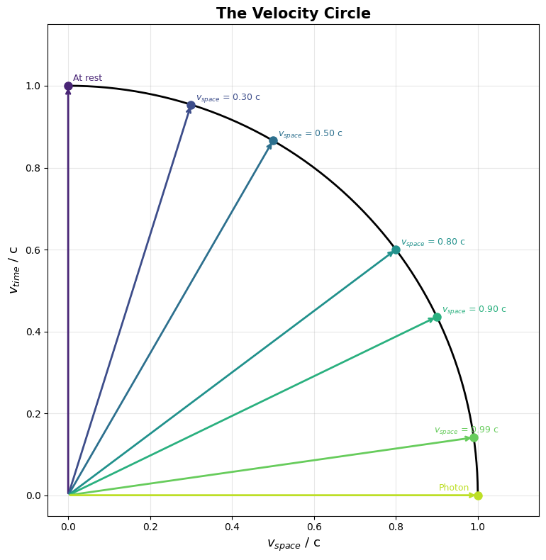
Core principle: every object always moves at exactly the speed of light \(c\) through four-dimensional spacetime. Time is a direction of motion just like the three spatial dimensions. An object at rest moves at 1 second per second through time — and that is the speed of light \(c\). Accelerating through space means rotating the velocity vector from the time direction toward the space direction.
This single principle reproduces all kinematic effects of special relativity: time dilation, length contraction, the Lorentz transformation, velocity addition and rapidity.
1.1 Direction θ and the velocity circle#
The velocity norm#
This is the equation of a 4D sphere with radius \(c\) in velocity space (shown here as a 2D cross-section in the direction of motion). The angle \(\theta\) measures the direction of the velocity vector relative to the time axis.
Parameterization with θ#
\(\theta = 0\): object at rest, moving at \(c\) through time
\(\theta = 90°\): photon, moving at \(c\) through space, no progress through time
Time dilation — directly from the geometry#
The proper time \(\tau\) of a moving object ticks slower by a factor \(\cos\theta\). This follows directly from the velocity circle: when a larger fraction of the velocity vector points into space, the component in the time direction is smaller.
# The Velocity Sphere (2D cross-section)
velocity_circle(lang='en')
pass
1.2 The moving observer#
Light moves at c for everyone#
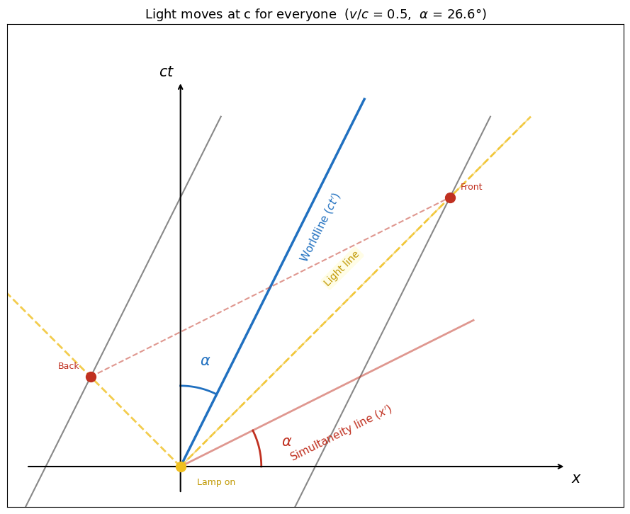
An astronaut in a moving spaceship turns on a lamp in the middle. She sees the light hit the front and back simultaneously — after all, the light moves at \(c\) in both directions, and the distances are equal.
An observer on the platform also sees the same light move at \(c\) — but the ship is moving. The back wall moves toward the light, the front wall moves away. The light reaches the back before the front.
Two events that are simultaneous for the astronaut are not simultaneous for the platform observer. This is the relativity of simultaneity — a direct consequence of the fact that both observers see light move at the same speed \(c\).
Duality: simultaneity and co-locality#
The spacetime diagram below shows the worldlines of the ship and the light rays from the lamp. The line through the two arrival events is the simultaneity line (\(x'\)-axis) of the astronaut — for her those two events happen at the same time. The worldline of the ship is the co-locality line (\(ct'\)-axis) — for her that is always the same place.
Both axes tilt by the same angle \(\alpha = \arctan(v/c)\): the worldline from the \(ct\)-axis, the simultaneity line from the \(x\)-axis. They are symmetric around the light line.
# Light in the spaceship: simultaneous for the astronaut, not for the platform
light_ship_diagram(beta=0.5, lang='en')
pass
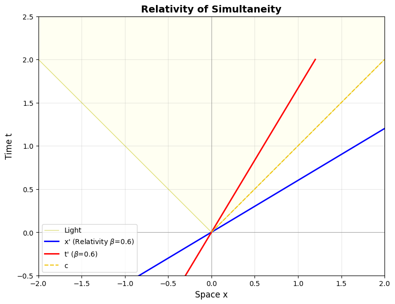
Relativity of simultaneity#
Two events that are simultaneous in S (\(\Delta t = 0\)) but separated by distance \(\Delta x\), are not simultaneous in S’ (\(v = c\sin\theta\)). The time difference is:
This is the special case (\(\Delta t = 0\)) of the general Lorentz time transformation (formula 6b below).
Length contraction#
The same \(\cos\theta\) geometry as time dilation applies to length measurement. A rod with rest length \(L_0\) is in spacetime a bundle of two parallel worldlines (front and back), separated perpendicularly by \(L_0\).
At velocity \(v = c\sin\theta\) the worldlines tilt by angle \(\theta\). The observer measures the distance between the endpoints at the same moment — a horizontal slice through spacetime. Two parallel lines at angle \(\theta\), with perpendicular separation \(L_0\), give a distance:
Time dilation and length contraction are the same geometry: projection of a unit vector onto the observer’s axis. This is summarized visually in §1.3.
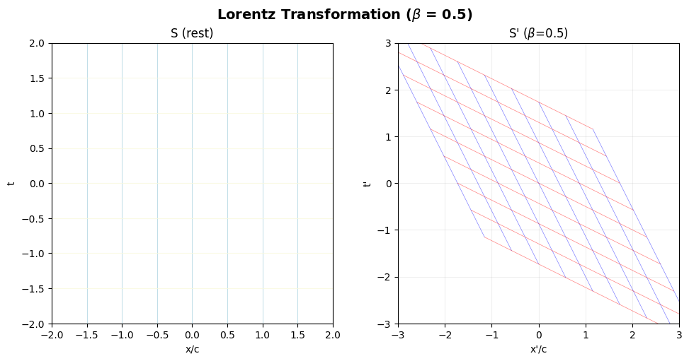
The full Lorentz transformation#
The four ingredients are:
Time dilation (\(\tau = t\cos\theta\))
Length contraction (\(L = L_0\cos\theta\))
Relativity of simultaneity (\(\Delta t' = (\tan\theta/c)\,\Delta x\) when \(\Delta t = 0\))
Galilean base shift (\(x - c\sin\theta \cdot t\))
Together they give:
This is identical to the Lorentz transformation from SRT: \(x' = \gamma(x - vt)\) and \(t' = \gamma(t - vx/c^2)\).
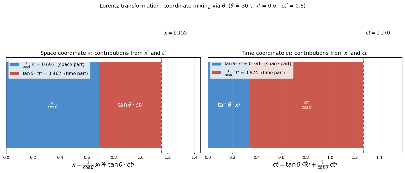
Inverse Lorentz transformation#
The inverse transformation (from the moving frame back to the rest frame) follows by \(\theta \to -\theta\) (the motion is reversed):
The coordinates mix: \(x\) depends on both \(x'\) and \(t'\), and vice versa. Written as a linear combination:
The diagonal is \(1/\cos\theta = \gamma\), the cross terms contain \(\tan\theta\). This is the hyperbolic “rotation” of spacetime — analogous to an ordinary rotation, but with \(\cosh\) and \(\sinh\) (via rapidity \(\varphi = \text{artanh}(\sin\theta)\)).
# Relativity of simultaneity
simultaneity_diagram(beta=0.6, lang='en')
pass
# Lorentz transformation: how the spacetime grid deforms
lorentz_transform_grid(beta=0.5, lang='en')
pass
# Numerical verification of the Lorentz transformation
beta = 0.6
stv = ORT.from_beta(beta)
v = stv.v_space
gamma = stv.gamma

print(f"Lorentz transformation for beta = {beta}, gamma = {gamma:.6f}")
print(f"v = {v:.2f} m/s\n")

# Test events (x in light-meters, t in seconds)
events = [
    (0, 0, "Origin"),
    (C, 0, "x=c, t=0 (simultaneous but not co-located)"),
    (0, 1, "x=0, t=1 (co-located but not simultaneous)"),
    (C, 1, "x=c, t=1"),
]

print(f"{'Event':<50} {'x':>12} {'t':>12} {'x_prime':>14} {'t_prime':>14}")
print("-" * 105)
for x, t, label in events:
    x_p, t_p = stv.lorentz_transform(x, t)
    # Verification with Einstein's formulas
    x_e = EinsteinModel.lorentz_x(x, t, v)
    t_e = EinsteinModel.lorentz_t(x, t, v)
    print(f"{label:<50} {x/C:12.4f}c {t:12.4f}s {x_p/C:14.4f}c {t_p:14.4f}s")
    assert abs(x_p - x_e) < 1e-6, "Mismatch!"
    assert abs(t_p - t_e) < 1e-6, "Mismatch!"

print("\nAll values match Einstein's Lorentz transformation exactly.")
Lorentz transformation for beta = 0.6, gamma = 1.250000
v = 179875474.80 m/s

Event                                                         x            t        x_prime        t_prime
---------------------------------------------------------------------------------------------------------
Origin                                                   0.0000c       0.0000s         0.0000c         0.0000s
x=c, t=0 (simultaneous but not co-located)               1.0000c       0.0000s         1.2500c        -0.7500s
x=0, t=1 (co-located but not simultaneous)               0.0000c       1.0000s        -0.7500c         1.2500s
x=c, t=1                                                 1.0000c       1.0000s         0.5000c         0.5000s

All values match Einstein's Lorentz transformation exactly.
# Coordinate mixing: how x and ct each consist of a space part and a time part
lorentz_decomposition_diagram(theta_deg=30, lang='en')
pass
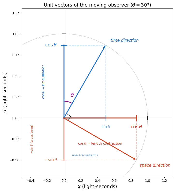
1.3 The unit circle#
The moving observer has their own time and space directions. These are perpendicular to each other and rotated by an angle \(\theta\) relative to the stationary observer.
In the diagram below these two directions are drawn as unit vectors on a circle with radius 1:
The time direction (blue) projects onto the stationary observer’s time axis with \(\cos\theta\) → time dilation
The space direction (red) projects onto the stationary observer’s space axis with \(\cos\theta\) → length contraction
Both effects are the same geometry: the projection of a unit vector of the moving observer onto the corresponding axis of the stationary observer always gives \(\cos\theta\).
# Unit vectors of the moving observer: both projections give cos(theta)
observer_axes_diagram(theta_deg=30, lang='en')
pass
1.4 Velocity addition#
In Newton’s mechanics velocities simply add: \(v_{total} = v_1 + v_2\). This violates the light-speed barrier.
The ORT formula via rapidities (see §1.5) gives:
This is identical to the relativistic velocity addition from SRT. Result: two objects each moving at \(0.8c\) see each other not at \(1.6c\) but at \(\approx 0.976c\) — always below \(c\).
# Velocity addition: 0.8c + 0.8c does NOT give 1.6c
v1 = 0.8 * C
v2 = 0.8 * C

v_newton = NewtonModel.velocity_addition(v1, v2)
v_srt = EinsteinModel.velocity_addition(v1, v2)
v_ort = ORT.velocity_addition(v1, v2)

print(f"Velocity addition: {v1/C:.1f}c + {v2/C:.1f}c")
print(f"  Newton:  {v_newton/C:.4f}c  (WRONG: exceeds c!)")
print(f"  SRT:     {v_srt/C:.4f}c")
print(f"  ORT:     {v_ort/C:.4f}c  (= SRT)")
print()

# Rapidity verification -- SRT and ORT
phi1_srt = math.atanh(v1 / C)
phi2_srt = math.atanh(v2 / C)
phi_total_srt = phi1_srt + phi2_srt
v_from_phi_srt = C * math.tanh(phi_total_srt)

phi1_ort = ORT.rapidity(v1)
phi2_ort = ORT.rapidity(v2)
phi_total_ort = phi1_ort + phi2_ort
v_from_phi_ort = C * math.tanh(phi_total_ort)

print(f"Rapidity (SRT): phi1={phi1_srt:.4f} + phi2={phi2_srt:.4f} = {phi_total_srt:.4f}")
print(f"  v = c*tanh(phi_total) = {v_from_phi_srt/C:.4f}c")
print(f"Rapidity (ORT): phi1={phi1_ort:.4f} + phi2={phi2_ort:.4f} = {phi_total_ort:.4f}")
print(f"  v = c*tanh(phi_total) = {v_from_phi_ort/C:.4f}c")
print(f"  Difference SRT vs ORT: {abs(phi_total_srt - phi_total_ort):.2e}  (identical)")
Velocity addition: 0.8c + 0.8c
  Newton:  1.6000c  (WRONG: exceeds c!)
  SRT:     0.9756c
  ORT:     0.9756c  (= SRT)

Rapidity (SRT): phi1=1.0986 + phi2=1.0986 = 2.1972
  v = c*tanh(phi_total) = 0.9756c
Rapidity (ORT): phi1=1.0986 + phi2=1.0986 = 2.1972
  v = c*tanh(phi_total) = 0.9756c
  Difference SRT vs ORT: 0.00e+00  (identical)
1.5 Rapidity#
The rapidity \(\varphi\) is the additive velocity parameter:
Rapidities are additive: \(\varphi_{total} = \varphi_1 + \varphi_2\).
The relativistic velocity addition formula (7) follows from this via \(v = c \tanh(\varphi)\).
Rapidity is the standard term in relativistic physics (e.g. Rindler, Jackson).
2 Invariance of Being#
Principle: the product of an object’s mass and its velocity through time is independent of the observer: \(m \cdot v_t = m_0 \cdot c\).
The name Ontological Relativity Theory refers to this concept: ontology is the philosophical study of what exists. ORT starts from Being — the fundamental existence of an object (\(m_0\)) — as an invariant.
When an object moves faster through space and thus slower through time, its mass increases proportionally, so that the product \(m \cdot v_t\) remains unchanged.
2.1 The Being principle#
Mass-Being (invariant)#
Energy corollary (derived)#
This follows directly from (8) and \(E = m_{rel} c^2\).
Relativistic mass#
From \(S_m = m_0 c\) and \(v_{time} = c\cos\theta\) follows:
The relativistic mass follows directly from the Being principle. In SRT the same result (\(\gamma m_0\)) is reached via momentum conservation under the Lorentz transformation.
# Verification: Invariance of Being for various velocities
m0 = 1.0  # kg (unit mass)
print(f"Invariance of Being: S_m = m_rel * v_time = m0 * c = {m0 * C:.6e} kg*m/s")
print()
print(f"{'beta':>6}  {'m_rel (gamma*m0)':>16}  {'v_time (m/s)':>14}  {'S_m':>14}  {'= m0*c?':>10}")
print("-" * 70)
for beta in [0.0, 0.3, 0.5, 0.8, 0.9, 0.99]:
    stv = ORT.from_beta(beta)
    m_rel = stv.relativistic_mass(m0)
    v_t = stv.v_time
    s_m = m_rel * v_t
    match = abs(s_m - m0 * C) < 1e-6
    print(f"{beta:6.2f}  {m_rel:16.6f}  {v_t:14.2f}  {s_m:14.6e}  {'YES' if match else 'NO':>10}")

print()
print("The Being value is constant -- independent of velocity!")
Invariance of Being: S_m = m_rel * v_time = m0 * c = 2.997925e+08 kg*m/s

  beta  m_rel (gamma*m0)    v_time (m/s)             S_m     = m0*c?
----------------------------------------------------------------------
  0.00          1.000000    299792458.00    2.997925e+08         YES
  0.30          1.048285    285983777.98    2.997925e+08         YES
  0.50          1.154701    259627884.49    2.997925e+08         YES
  0.80          1.666667    179875474.80    2.997925e+08         YES
  0.90          2.294157    130676502.85    2.997925e+08         YES
  0.99          7.088812     42290930.54    2.997925e+08         YES

The Being value is constant -- independent of velocity!
2.2 The work integral#
The factor \(c^2\) follows from the mathematics. The key is the standard definition of kinetic energy as work:
We know \(v\) and \(p\) both as functions of \(\theta\):
The origin of \(c^2\): the product \(v \cdot dp\) contains \(c \cdot c\): one \(c\) from velocity \(v = c\sin\theta\), one \(c\) from momentum \(p = m_0 c \tan\theta\). The factor \(c^2\) is a computational consequence.
The total energy is:
At rest (\(\theta = 0\)) this reduces to \(E_0 = m_0 c^2\).
Being for energy#
The product \(E \cdot v_t\) is also invariant — a direct consequence of Mass-Being.
# Numerical verification: work integral E_kin = integral(v dp) = (gamma - 1) m0 c^2
# This is the NON-CIRCULAR derivation of E = mc^2 (§4.4)
m0 = 1.0  # kg

print("Work integral: E_kin = ∫ v dp = m₀c² (1/cos(θ) - 1)")
print(f"{'':>58} {'Numerical':>14} {'Analytical':>14} {'Difference':>14}")
print("-" * 100)

for beta in [0.1, 0.3, 0.5, 0.8, 0.9, 0.95, 0.99]:
    stv = ORT.from_beta(beta)

    # Numerical integral via the new method
    E_numerical = stv.kinetic_energy_integral(m0, n_steps=1_000_000)

    # Analytical result: (gamma - 1) m0 c^2
    E_analytical = stv.kinetic_energy(m0)

    rel_diff = abs(E_numerical - E_analytical) / E_analytical if E_analytical > 0 else 0

    print(f"  β = {beta:.2f}  θ = {math.degrees(stv.theta):6.2f}°  γ = {stv.gamma:8.4f}  "
          f"{E_numerical:14.6e} {E_analytical:14.6e} {rel_diff:14.2e}")

print()
print("The numerical work integral matches the analytical result.")
print("c² arises as c · c: one c from v = c·sin(θ), one c from p = m₀c·tan(θ).")
Work integral: E_kin = ∫ v dp = m₀c² (1/cos(θ) - 1)
                                                                Numerical     Analytical     Difference
----------------------------------------------------------------------------------------------------
β = 0.10 θ = 5.74° γ = 1.0050 4.527763e+14 4.527763e+14 3.06e-14
β = 0.30 θ = 17.46° γ = 1.0483 4.339625e+15 4.339625e+15 2.56e-14
β = 0.50 θ = 30.00° γ = 1.1547 1.390379e+16 1.390379e+16 6.47e-14
β = 0.80 θ = 53.13° γ = 1.6667 5.991701e+16 5.991701e+16 3.59e-13
β = 0.90 θ = 64.16° γ = 2.2942 1.163131e+17 1.163131e+17 8.31e-13
β = 0.95 θ = 71.81° γ = 3.2026 1.979565e+17 1.979565e+17 1.83e-12
  β = 0.99  θ =  81.89°  γ =   7.0888    5.472351e+17   5.472351e+17       9.84e-12

The numerical work integral matches the analytical result.
c² arises as c · c: one c from v = c·sin(θ), one c from p = m₀c·tan(θ).
# Verification: energy-momentum relation E^2 = (pc)^2 + (m0*c^2)^2
m0 = 1.0  # kg
print("Energy-momentum relation (equation 16):")
print(f"  m0*c^2 = {m0 * C**2:.6e} J\n")

for beta in [0.0, 0.5, 0.8, 0.99]:
    stv = ORT.from_beta(beta)
    E = stv.total_energy(m0)
    p = stv.momentum(m0)
    lhs = E**2
    rhs = (p * C)**2 + (m0 * C**2)**2
    print(f"  beta={beta:.2f}: E={E:.6e} J, p={p:.6e} kg*m/s")
    print(f"    E^2              = {lhs:.6e}")
    print(f"    (pc)^2+(m0c^2)^2 = {rhs:.6e}")
    print(f"    Match: {abs(lhs - rhs) / lhs < 1e-12}\n")
Energy-momentum relation (equation 16):
  m0*c^2 = 8.987552e+16 J

  beta=0.00: E=8.987552e+16 J, p=0.000000e+00 kg*m/s
    E^2              = 8.077609e+33
    (pc)^2+(m0c^2)^2 = 8.077609e+33
    Match: True

  beta=0.50: E=1.037793e+17 J, p=1.730853e+08 kg*m/s
    E^2              = 1.077014e+34
    (pc)^2+(m0c^2)^2 = 1.077014e+34
    Match: True

  beta=0.80: E=1.497925e+17 J, p=3.997233e+08 kg*m/s
    E^2              = 2.243780e+34
    (pc)^2+(m0c^2)^2 = 2.243780e+34
    Match: True

  beta=0.99: E=6.371107e+17 J, p=2.103921e+09 kg*m/s
    E^2              = 4.059100e+35
    (pc)^2+(m0c^2)^2 = 4.059100e+35
    Match: True
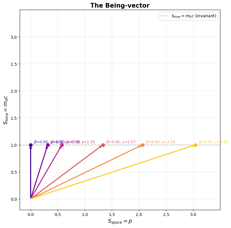
2.3 The Being-vector#
The Being-vector \(\vec{S}\) has two components:
Being is time-momentum. The structure is symmetric:
Through space |
Through time |
|
|---|---|---|
Velocity |
\(v = c\sin\theta\) |
\(d\tau/dt = \cos\theta\) |
“Momentum” |
\(p = m_{rel} \cdot v\) |
\(m_{rel} \cdot d\tau/dt = m_0\) |
The magnitude of the Being-vector:
Pythagoras on the Being-vector gives the energy-momentum relation:
# Being-vector diagram
zijn_vector_diagram(lang='en')
pass
2.4 The four-momentum#
The Being-vector contains the same physics as the four-momentum \(p^\mu\) from SRT, but the presentation differs fundamentally:
Component |
Four-momentum \(p^\mu\) (SRT) |
Being-vector \(\vec{S}\) (ORT) |
|---|---|---|
Space |
\(p\) |
\(S_{space} = p\) |
Time |
\(p^0 = E/c\) |
\(S_{time} = m_0 c\) |
Magnitude |
\(m_0 c\) (as norm) |
\(\lvert\vec{S}\rvert = E/c\) |
The four-momentum hides \(m_0\) as a norm — you need to compute \(\sqrt{p^\mu p_\mu}\) to recover the rest mass. The Being-vector makes the invariance of \(m_0\) directly visible as a component: \(S_{time} = m_0 c\) is right there.
Physical interpretation#
Why mass increases: the Being-vector rotates with increasing speed, but \(S_{time} = m_0 c\) remains constant. Since \(v_{time}\) decreases, \(m_{rel}\) must increase to maintain the product.
Light barrier: as \(\theta \to 90°\), \(m_{rel} \to \infty\). Infinite energy is needed to accelerate a massive object to \(c\).
Photons: \(\theta = 90°\), \(m_0 = 0\), \(S_{time} = 0\). The Being-vector points entirely in the space direction: \(|\vec{S}| = p = E/c\).
The derivation chain#
3 ORT and SRT compared#
ORT and Einstein’s SRT are mathematically equivalent — they describe the same physics. The difference lies in the starting point and the interpretation.
ORT starts from the geometry of the velocity circle (\(\theta\)) and Invariance of Being. SRT starts from the relativity principle and the constancy of \(c\). Both lead to identical formulas.
3.1 Formula overview#
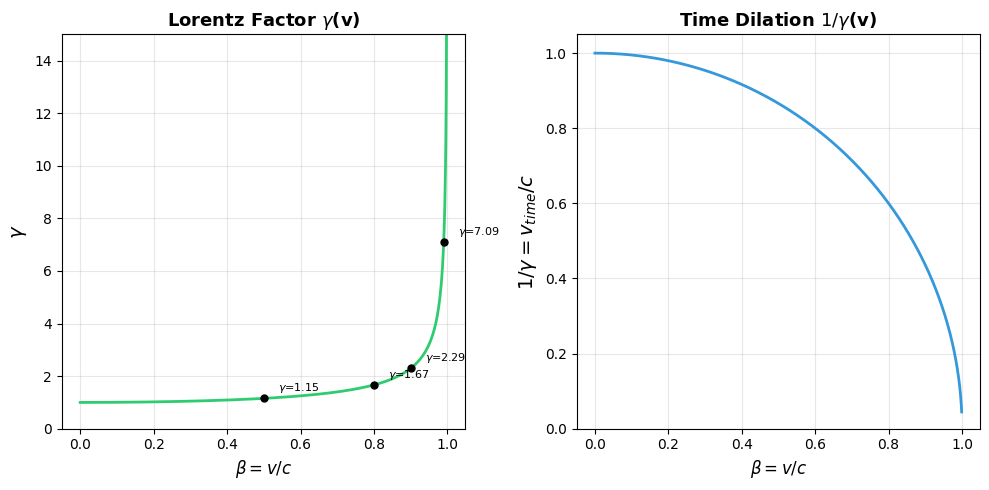
The Lorentz factor#
The Lorentz factor from SRT is simply the secant of \(\theta\). In ORT, \(\gamma\) is a derived quantity, not the fundamental starting point.
Energy#
Momentum#
Complete formula table#
Nr |
Name |
ORT (\(\theta\)) |
Being formula |
Interpretation |
|---|---|---|---|---|
(1) |
Velocity norm |
\(v_r^2 + v_t^2 = c^2\) |
— |
Everything moves at \(c\) |
(2) |
Components |
\(v_r = c\sin\theta\), \(v_t = c\cos\theta\) |
— |
Direction determines distribution |
(3) |
Time dilation |
\(d\tau/dt = \cos\theta\) |
— |
Projection onto time axis |
(5) |
Length contraction |
\(L = L_0\cos\theta\) |
— |
Projection onto space axis |
(8) |
Being (time) |
\(m_0 c\) |
\(m_{rel} \cdot v_t\) |
Invariant |
(10) |
Rel. mass |
\(m_0/\cos\theta\) |
from (8) |
From Invariance of Being |
(12) |
Total energy |
\(m_0 c^2/\cos\theta\) |
from (10) + integral |
Mass × \(c^2\) |
(17) |
Lorentz factor |
\(1/\cos\theta\) |
— |
Secant of \(\theta\) |
(19) |
Kinetic energy |
\((1/\cos\theta - 1)\,m_0 c^2\) |
from (11) |
Work done |
(20) |
Momentum |
\(m_0 c\tan\theta\) |
\(m_{rel} \cdot v\) |
Spatial momentum |
# Gamma curve: how gamma increases with velocity
gamma_curve(lang='en')
pass
# Compute gamma for various velocities
print(f"{'beta':>8}  {'theta (degrees)':>15}  {'gamma':>10}  {'v_time/c':>10}")
print("-" * 50)
for beta in [0.0, 0.1, 0.3, 0.5, 0.8, 0.9, 0.95, 0.99, 0.999]:
    stv = ORT.from_beta(beta)
    print(f"{beta:8.3f}  {math.degrees(stv.theta):15.2f}  {stv.gamma:10.4f}  {stv.v_time/C:10.6f}")
    beta  theta (degrees)       gamma    v_time/c
--------------------------------------------------
   0.000             0.00      1.0000    1.000000
   0.100             5.74      1.0050    0.994987
   0.300            17.46      1.0483    0.953939
   0.500            30.00      1.1547    0.866025
   0.800            53.13      1.6667    0.600000
   0.900            64.16      2.2942    0.435890
   0.950            71.81      3.2026    0.312250
   0.990            81.89      7.0888    0.141067
   0.999            87.44     22.3663    0.044710
3.2 SRT formulas in ORT notation#
Formula |
SRT (\(\gamma, \beta\)) |
ORT (\(\theta\)) |
|---|---|---|
Time dilation |
\(\tau = t/\gamma\) |
\(\tau = t\cos\theta\) |
Length contraction |
\(L = L_0/\gamma\) |
\(L = L_0\cos\theta\) |
Rel. mass |
\(\gamma m_0\) |
\(m_0/\cos\theta\) |
Momentum |
\(\gamma m_0 v\) |
\(m_0 c\tan\theta\) |
Total energy |
\(\gamma m_0 c^2\) |
\(m_0 c^2/\cos\theta\) |
Kinetic energy |
\((\gamma-1)m_0 c^2\) |
\((1/\cos\theta - 1)m_0 c^2\) |
Velocity addition |
\(\frac{v_1+v_2}{1+v_1v_2/c^2}\) |
idem (via rapidity) |
Lorentz transf. (x) |
\(\gamma(x-vt)\) |
\((x - c\sin\theta \cdot t)/\cos\theta\) |
Lorentz transf. (t) |
\(\gamma(t-vx/c^2)\) |
\((t - \sin\theta \cdot x/c)/\cos\theta\) |
Simultaneity |
\(\gamma v \Delta x/c^2\) |
\((\tan\theta/c)\Delta x\) |
Energy-momentum |
\(E^2 = (pc)^2 + (m_0c^2)^2\) |
idem (Pythagoras on \(\vec{S}\)) |
Rapidity |
\(\text{artanh}(\beta)\) |
\(\text{artanh}(\sin\theta)\) |
All formulas are identical — the only difference is notation. \(\gamma = 1/\cos\theta\) and \(\beta = \sin\theta\) translate directly between both.
3.3 Newton, Einstein and ORT#
Aspect |
Newton |
Einstein (SRT) |
ORT |
|---|---|---|---|
Time dilation |
None |
\(\tau = t/\gamma\) |
\(\tau = t\cos\theta\) |
Length contraction |
None |
\(L = L_0/\gamma\) |
\(L = L_0\cos\theta\) |
Velocity addition |
\(v_1 + v_2\) |
Relativistic |
Idem (rapidities) |
Mass |
Constant \(m\) |
\(\gamma m_0\) |
\(m_0/\cos\theta\) from Being |
\(E = mc^2\) |
— |
Derived (Lorentz + momentum conservation) |
Derived (Invariance of Being) |
Newton diverges fundamentally at high velocities. Einstein (SRT) and ORT give identical numerical results — they describe the same physics.
# Relativistic effects at v = 0.8c -- Newton vs SRT vs ORT
beta = 0.8
v = beta * C
stv = ORT.from_beta(beta)
m0 = 1.0  # kg
L0 = 1.0  # m (rest length)
t_coord = 1.0  # s (coordinate time)
theta_deg = math.degrees(stv.theta)

print(f"=== Relativistic effects at beta = {beta} ===")
print(f"  theta = {theta_deg:.2f} degrees,  gamma = {stv.gamma:.6f}")
print()

# --- Time dilation ---
td_newton = NewtonModel.proper_time(t_coord, v)
td_srt = EinsteinModel.proper_time(t_coord, v)
td_ort = stv.proper_time(t_coord)

print(f"Time dilation (tau for t = {t_coord} s):")
print(f"  {'Newton':>8}: {td_newton:.6f} s  (no dilation)")
print(f"  {'SRT':>8}: {td_srt:.6f} s  (= t/gamma)")
print(f"  {'ORT':>8}: {td_ort:.6f} s  (= t*cos(theta))")
print()

# --- Length contraction ---
lc_newton = L0  # Newton: no contraction
lc_srt = EinsteinModel.length(L0, v)
lc_ort = stv.length_contraction(L0)

print(f"Length contraction (L0 = {L0} m):")
print(f"  {'Newton':>8}: {lc_newton:.6f} m  (no contraction)")
print(f"  {'SRT':>8}: {lc_srt:.6f} m  (= L0/gamma)")
print(f"  {'ORT':>8}: {lc_ort:.6f} m  (= L0*cos(theta))")
print()

# --- Momentum ---
p_newton = NewtonModel.momentum(m0, v)
p_srt = EinsteinModel.momentum(m0, v)
p_ort = stv.momentum(m0)

print(f"Momentum (m0 = {m0} kg):")
print(f"  {'Newton':>8}: {p_newton:.6e} kg*m/s  (= m0*v)")
print(f"  {'SRT':>8}: {p_srt:.6e} kg*m/s  (= gamma*m0*v)")
print(f"  {'ORT':>8}: {p_ort:.6e} kg*m/s  (= m0*c*tan(theta))")
print()

# --- Kinetic energy ---
ek_newton = NewtonModel.kinetic_energy(m0, v)
ek_srt = EinsteinModel.kinetic_energy(m0, v)
ek_ort = stv.kinetic_energy(m0)

print(f"Kinetic energy:")
print(f"  {'Newton':>8}: {ek_newton:.6e} J  (= 0.5*m0*v^2)")
print(f"  {'SRT':>8}: {ek_srt:.6e} J  (= (gamma-1)*m0*c^2)")
print(f"  {'ORT':>8}: {ek_ort:.6e} J  (= (1/cos(theta)-1)*m0*c^2)")
print()

# --- Verification SRT = ORT ---
print("Verification SRT = ORT:")
print(f"  Time dilation:      diff = {abs(td_srt - td_ort):.2e}")
print(f"  Length contraction:  diff = {abs(lc_srt - lc_ort):.2e}")
print(f"  Momentum:            diff = {abs(p_srt - p_ort):.2e}")
print(f"  Kinetic energy:      diff = {abs(ek_srt - ek_ort):.2e}")
print("  SRT and ORT give identical results!")
=== Relativistic effects at beta = 0.8 ===
  theta = 53.13 degrees,  gamma = 1.666667

Time dilation (tau for t = 1.0 s):
    Newton: 1.000000 s  (no dilation)
       SRT: 0.600000 s  (= t/gamma)
       ORT: 0.600000 s  (= t*cos(theta))

Length contraction (L0 = 1.0 m):
    Newton: 1.000000 m  (no contraction)
       SRT: 0.600000 m  (= L0/gamma)
       ORT: 0.600000 m  (= L0*cos(theta))

Momentum (m0 = 1.0 kg):
    Newton: 2.398340e+08 kg*m/s  (= m0*v)
       SRT: 3.997233e+08 kg*m/s  (= gamma*m0*v)
       ORT: 3.997233e+08 kg*m/s  (= m0*c*tan(theta))

Kinetic energy:
    Newton: 2.876017e+16 J  (= 0.5*m0*v^2)
       SRT: 5.991701e+16 J  (= (gamma-1)*m0*c^2)
       ORT: 5.991701e+16 J  (= (1/cos(theta)-1)*m0*c^2)

Verification SRT = ORT:
  Time dilation:      diff = 1.11e-16
  Length contraction:  diff = 1.11e-16
  Momentum:            diff = 5.96e-08
  Kinetic energy:      diff = 1.60e+01
  SRT and ORT give identical results!
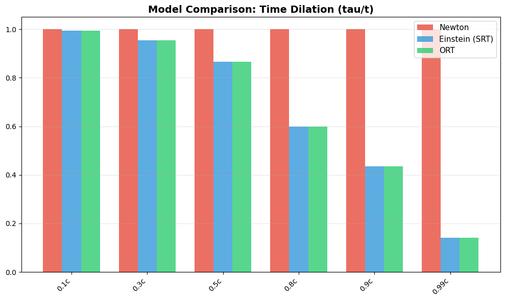
# Model comparison: time dilation at various velocities
betas_compare = [0.1, 0.3, 0.5, 0.8, 0.9, 0.99]
labels = [f'{b}c' for b in betas_compare]

newton_td = [1.0 for _ in betas_compare]  # Newton: no dilation
einstein_td = []
spacetime_td = []

for beta in betas_compare:
    v = beta * C
    stv = ORT.from_beta(beta)
    einstein_td.append(EinsteinModel.proper_time(1.0, v))
    spacetime_td.append(stv.proper_time(1.0))

values = {
    'labels': labels,
    'newton': newton_td,
    'einstein': einstein_td,
    'spacetime': spacetime_td
}
model_comparison_bar('Time Dilation (tau/t)', values, lang='en')
pass
# Detailed comparison table
m0 = 1.0  # kg
print(f"{'beta':>6} | {'Newton tau':>12} {'Einstein tau':>14} {'ORT tau':>14} | "
      f"{'Newton p':>14} {'Einstein p':>14} {'ORT p':>14}")
print("-" * 100)

for beta in [0.1, 0.3, 0.5, 0.8, 0.9, 0.95, 0.99]:
    v = beta * C
    stv = ORT.from_beta(beta)

    # Proper time for 1 second of coordinate time
    tau_n = NewtonModel.proper_time(1.0, v)
    tau_e = EinsteinModel.proper_time(1.0, v)
    tau_st = stv.proper_time(1.0)

    # Momentum
    p_n = NewtonModel.momentum(m0, v)
    p_e = EinsteinModel.momentum(m0, v)
    p_st = stv.momentum(m0)

    print(f"{beta:6.2f} | {tau_n:12.6f} {tau_e:14.6f} {tau_st:14.6f} | "
          f"{p_n:14.6e} {p_e:14.6e} {p_st:14.6e}")

print("\nEinstein (SRT) and ORT give identical results.")
print("Newton deviates increasingly at higher velocities.")
  beta |   Newton tau   Einstein tau        ORT tau |       Newton p     Einstein p          ORT p
----------------------------------------------------------------------------------------------------
  0.10 |     1.000000       0.994987       0.994987 |   2.997925e+07   3.013028e+07   3.013028e+07
  0.30 |     1.000000       0.953939       0.953939 |   8.993774e+07   9.428037e+07   9.428037e+07
  0.50 |     1.000000       0.866025       0.866025 |   1.498962e+08   1.730853e+08   1.730853e+08
  0.80 |     1.000000       0.600000       0.600000 |   2.398340e+08   3.997233e+08   3.997233e+08
  0.90 |     1.000000       0.435890       0.435890 |   2.698132e+08   6.189940e+08   6.189940e+08
  0.95 |     1.000000       0.312250       0.312250 |   2.848028e+08   9.120990e+08   9.120990e+08
  0.99 |     1.000000       0.141067       0.141067 |   2.967945e+08   2.103921e+09   2.103921e+09

Einstein (SRT) and ORT give identical results.
Newton deviates increasingly at higher velocities.
3.4 Three derivation paths#
How do Newton, Einstein, and ORT each arrive at the same relativistic formulas?
Step |
Newton |
Einstein (SRT) |
ORT |
|---|---|---|---|
Starting point |
Absolute space and time |
Relativity principle + \(c\) constant |
Everything moves at \(c\) + Invariance of Being |
Space and time |
Independent, universal |
Interwoven: spacetime |
Interwoven: velocity sphere |
Mass |
Constant |
Invariant rest mass; \(\gamma m_0\) in momentum |
\(m_0/\cos\theta\) from Being principle |
Momentum |
\(p = mv\) |
\(p = \gamma m_0 v\) (momentum conservation + Lorentz) |
\(p = m_0 c\tan\theta\) (from \(m_{rel} \cdot v\)) |
Energy |
\(E_k = \tfrac{1}{2}mv^2\) |
\(E = \gamma m_0 c^2\) (work integral) |
\(E = m_0 c^2/\cos\theta\) (work integral) |
Lorentz transf. |
Galilean: \(x' = x - vt\) |
From postulates (light-speed invariance) |
From velocity circle (simultaneity duality) |
The work integral \(E_k = \int v \, dp\) is identical in SRT and ORT — the difference lies only in how \(m_{rel}\) is motivated (Lorentz invariance of momentum vs. Invariance of Being).
3.5 Thought experiments#
Three classic tests of special relativity, computed with both SRT and ORT.
Twin Paradox#
Alice stays on Earth, Bob travels at \(v = 0.8c\) to a star 10 light-years away and back.
Muon Decay#
Muons are created at ~10 km altitude and move at \(v \approx 0.998c\). Without relativity they would decay after ~660 m.
GPS Correction (SRT part)#
GPS satellites move at ~3.87 km/s. Special relativity causes a measurable time delay.
# 9.1 Twin Paradox
print("=== Twin Paradox ===")
beta_bob = 0.8
distance_ly = 10  # light-years one way
stv_bob = ORT.from_beta(beta_bob)
theta_bob = math.degrees(stv_bob.theta)

t_alice_one_way = distance_ly / beta_bob
t_alice_total = 2 * t_alice_one_way

# ORT: proper time Bob = t * cos(theta)
t_bob_ort = t_alice_total * math.cos(stv_bob.theta)

# SRT: proper time Bob = t / gamma
t_bob_srt = t_alice_total / stv_bob.gamma

print(f"  Bob travels at {beta_bob}c to a star {distance_ly} light-years away")
print(f"  theta = {theta_bob:.2f} degrees")
print()
print(f"  Alice (Earth): {t_alice_total:.2f} years")
print(f"  Bob (ORT):  tau = t * cos(theta) = {t_alice_total:.2f} * cos({theta_bob:.2f}) = {t_bob_ort:.2f} years")
print(f"  Bob (SRT):  tau = t / gamma     = {t_alice_total:.2f} / {stv_bob.gamma:.4f}    = {t_bob_srt:.2f} years")
print(f"  Difference ORT vs SRT: {abs(t_bob_ort - t_bob_srt):.2e} years (identical)")
print()
print(f"  Bob is {t_alice_total - t_bob_ort:.2f} years younger upon return")
=== Twin Paradox ===
  Bob travels at 0.8c to a star 10 light-years away
  theta = 53.13 degrees

  Alice (Earth): 25.00 years
  Bob (ORT):  tau = t * cos(theta) = 25.00 * cos(53.13) = 15.00 years
  Bob (SRT):  tau = t / gamma     = 25.00 / 1.6667    = 15.00 years
  Difference ORT vs SRT: 0.00e+00 years (identical)

  Bob is 10.00 years younger upon return
# 9.2 Muon Decay
print("=== Muon Decay ===")
beta_muon = 0.998
tau_muon = 2.2e-6  # rest lifetime in seconds
h_atmosphere = 10000  # height in meters

stv_muon = ORT.from_beta(beta_muon)
theta_muon = math.degrees(stv_muon.theta)

d_classical = beta_muon * C * tau_muon

# ORT: lifetime = tau / cos(theta)
t_ort = tau_muon / math.cos(stv_muon.theta)
d_ort = beta_muon * C * t_ort

# SRT: lifetime = tau * gamma
t_srt = tau_muon * stv_muon.gamma
d_srt = beta_muon * C * t_srt

print(f"  Muon speed: {beta_muon}c, theta = {theta_muon:.2f} degrees")
print(f"  Rest lifetime: {tau_muon*1e6:.1f} microseconds")
print()
print(f"  Without relativity:")
print(f"    Distance = {d_classical:.0f} m ({d_classical/1000:.2f} km) -- does NOT reach ground")
print()
print(f"  ORT: lifetime = tau / cos(theta) = {t_ort*1e6:.1f} us")
ort_reaches = "YES" if d_ort > h_atmosphere else "NO"
print(f"    Distance = {d_ort/1000:.1f} km -- reaches ground: {ort_reaches}")
print()
print(f"  SRT: lifetime = tau * gamma      = {t_srt*1e6:.1f} us")
srt_reaches = "YES" if d_srt > h_atmosphere else "NO"
print(f"    Distance = {d_srt/1000:.1f} km -- reaches ground: {srt_reaches}")
print()
print(f"  Difference ORT vs SRT: {abs(d_ort - d_srt):.2e} m (identical)")
=== Muon Decay ===
  Muon speed: 0.998c, theta = 86.38 degrees
  Rest lifetime: 2.2 microseconds

  Without relativity:
    Distance = 658 m (0.66 km) -- does NOT reach ground

  ORT: lifetime = tau / cos(theta) = 34.8 us
    Distance = 10.4 km -- reaches ground: YES

  SRT: lifetime = tau * gamma      = 34.8 us
    Distance = 10.4 km -- reaches ground: YES

  Difference ORT vs SRT: 0.00e+00 m (identical)
# 9.3 GPS SRT correction
print("=== GPS Special Relativity Correction ===")
v_gps = 3870  # m/s (GPS satellite orbital speed)
stv_gps = ORT.from_v(v_gps)
theta_gps = stv_gps.theta
seconds_per_day = 86400

# ORT: proper time = t * cos(theta)
tau_ort = seconds_per_day * math.cos(theta_gps)
delta_ort = seconds_per_day - tau_ort

# SRT: proper time = t / gamma
tau_srt = seconds_per_day / stv_gps.gamma
delta_srt = seconds_per_day - tau_srt

print(f"  Orbital speed: {v_gps} m/s")
print(f"  theta = {math.degrees(theta_gps):.6f} degrees")
print()
print(f"  ORT: tau = t * cos(theta)")
print(f"    Time delay per day: {delta_ort*1e9:.2f} nanoseconds")
print()
print(f"  SRT: tau = t / gamma")
print(f"    Time delay per day: {delta_srt*1e9:.2f} nanoseconds")
print()
print(f"  Difference ORT vs SRT: {abs(delta_ort - delta_srt)*1e9:.4f} ns (identical)")
print()
print(f"  Satellite clock runs SLOWER due to motion (SRT).")
print(f"  (Note: GRT causes a SPEEDUP due to less gravity, which is larger.)")
=== GPS Special Relativity Correction ===
  Orbital speed: 3870 m/s
  theta = 0.000740 degrees

  ORT: tau = t * cos(theta)
    Time delay per day: 7198.86 nanoseconds

  SRT: tau = t / gamma
    Time delay per day: 7198.86 nanoseconds

  Difference ORT vs SRT: 0.0000 ns (identical)

  Satellite clock runs SLOWER due to motion (SRT).
  (Note: GRT causes a SPEEDUP due to less gravity, which is larger.)